How to Convert Time Zones in Excel (Formulas That Handle DST)

To convert a time zone in Excel, add or subtract the difference in hours divided by 24, because Excel stores one day as 1. With a UTC time in A2, =A2-5/24 gives New York winter time (EST), =A2+5.5/24 gives India time, and =A2+9/24 gives Tokyo. A fixed offset is wrong for part of the year in any zone with daylight saving time, so below there is a formula that knows the switch dates for the US and Europe.

We ran every formula on this page in Microsoft Excel for Mac (version 16.113) on 28 September 2026. The daylight saving formulas returned the same result as Python's time zone database for 256 UTC times from 2024 to 2030, including every hour around each switch.

We build Slack Green, a tool that keeps your Slack status green, and we work with a team spread across time zones. If you only need to check one time, our free time zone converter is faster than a spreadsheet.

The basic time zone formula in Excel

Excel stores a date and time as one number: the whole part is the day, the decimal part is the time of day. One hour is 1/24. To move a time to another zone, add or subtract the hours between the two zones:

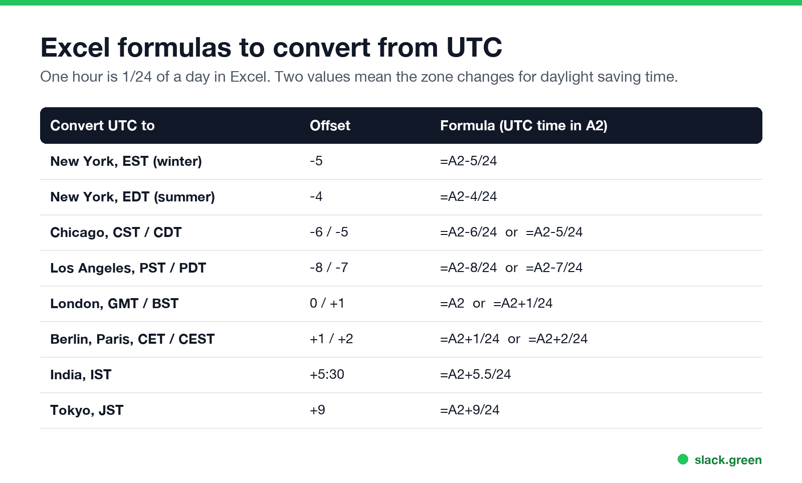
UTC to New York (EST, winter)   =A2-5/24
UTC to New York (EDT, summer)   =A2-4/24
UTC to India (IST)              =A2+5.5/24
New York (EDT) to Tokyo (JST)   =A2+13/24

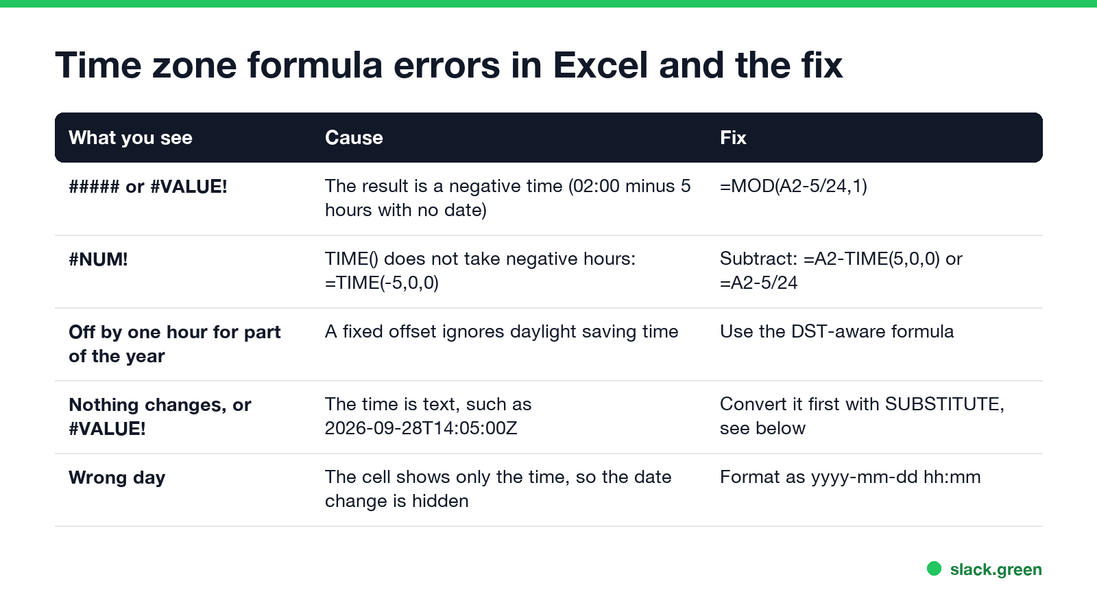
=A2-TIME(5,0,0) gives the same result as =A2-5/24. TIME() only takes 0 to 23 hours, so =TIME(-5,0,0) returns #NUM!; write a negative offset as a subtraction. For half-hour zones such as India, =A2+5.5/24 and =A2+TIME(5,30,0) both work: 2026-09-28 14:05 UTC became 19:35.

To go between two local zones, subtract the two UTC offsets. New York in summer is UTC-4 and Tokyo is UTC+9, so the difference is 9 - (-4) = 13 hours: =A2+13/24. In our test, 14:05 in New York became 03:05 the next day in Tokyo, and Excel moved the date on its own.

Format the result cell as a date and time (Format Cells, Custom, yyyy-mm-dd hh:mm). If the cell shows only hh:mm, a conversion that crosses midnight looks right but sits on the wrong day.

Convert time zones with a lookup table

If a sheet has many rows with different target zones, keep the offsets in a small table and look them up. Put zone names in D1:D4 and their UTC offsets in E1:E4:

D            E
New York    -4
London       1
India        5.5
Tokyo        9

Then, with the UTC time in A2 and the zone name in F1:

=A2+VLOOKUP(F1,$D$1:$E$4,2,FALSE)/24

With F1 set to India, 14:05 UTC returned 19:35. VLOOKUP works in every version of Excel and in Google Sheets. The offsets in this table are fixed, so update the New York and London rows when daylight saving time starts and ends, or use the formulas in the next section.

A formula that handles daylight saving time

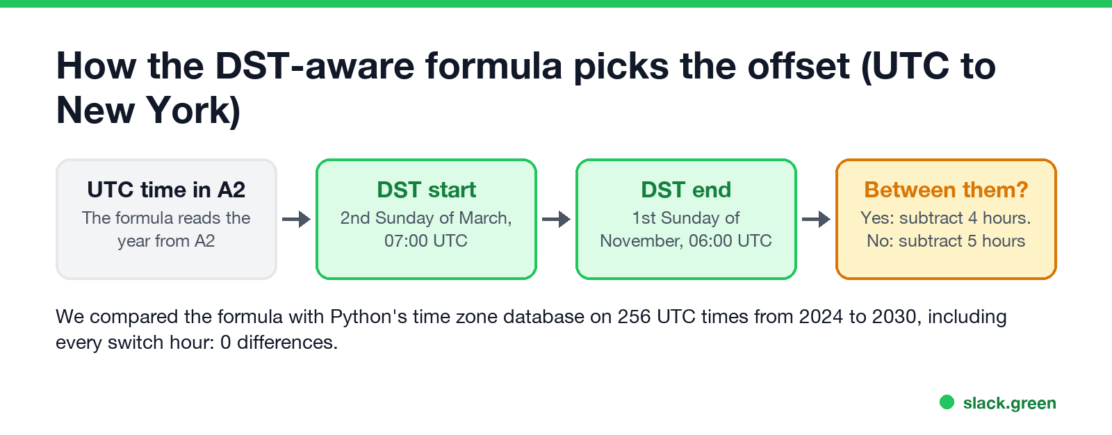
Excel has no time zone database, so no built-in function knows that New York is UTC-5 in winter and UTC-4 in summer. You can work out the switch dates with DATE and WEEKDAY. In the United States, daylight saving time starts on the second Sunday of March at 2:00 local time (07:00 UTC) and ends on the first Sunday of November at 2:00 local time (06:00 UTC).

UTC to New York, with the UTC time in A2:

=A2+IF(AND(A2>=DATE(YEAR(A2),3,8)+MOD(1-WEEKDAY(DATE(YEAR(A2),3,8)),7)+7/24,A2<DATE(YEAR(A2),11,1)+MOD(1-WEEKDAY(DATE(YEAR(A2),11,1)),7)+6/24),-4,-5)/24

DATE(YEAR(A2),3,8)+MOD(1-WEEKDAY(DATE(YEAR(A2),3,8)),7) is the first Sunday on or after 8 March, which is always the second Sunday of March. The November part finds the first Sunday on or after 1 November. For Chicago, change -4,-5 to -5,-6 and the switch times to 8/24 and 7/24. For Los Angeles use -7,-8 with 10/24 and 9/24.

In the EU and the UK, clocks change on the last Sunday of March and the last Sunday of October, both at 01:00 UTC. UTC to London:

=A2+IF(AND(A2>=DATE(YEAR(A2),3,31)-MOD(WEEKDAY(DATE(YEAR(A2),3,31))-1,7)+1/24,A2<DATE(YEAR(A2),10,31)-MOD(WEEKDAY(DATE(YEAR(A2),10,31))-1,7)+1/24),1,0)/24

For Berlin, Paris, Madrid or Rome, change 1,0 to 2,1. We filled a sheet with 256 UTC times, including 7 times around each switch in every year from 2024 to 2030, and ran the New York, London and Berlin formulas. All 768 results matched Python's zoneinfo.

These formulas use only IF, AND, DATE, YEAR, WEEKDAY and MOD, so they work in old versions of Excel too. They follow the current rules; if a country changes its daylight saving dates, the formula needs the new dates. Zones without daylight saving time, such as India, Japan, China and most of Arizona, need only the fixed offset.

Convert a text timestamp such as 2026-09-28T14:05:00Z

Timestamps exported from apps and APIs often arrive as text in ISO 8601 format. Excel does not treat 2026-09-28T14:05:00Z as a date until you remove the T and the Z:

=--SUBSTITUTE(SUBSTITUTE(A2,"T"," "),"Z","")

The two minus signs turn the text into a number. Add the offset as usual: =--SUBSTITUTE(SUBSTITUTE(A2,"T"," "),"Z","")-4/24 returned 2026-09-28 10:05 for New York. Unix timestamps (seconds since 1970) need a different formula, covered in how to convert a Unix timestamp to a date in Excel.

Convert only the time, without a date

If a cell holds only a time, such as 02:00, subtracting five hours gives a negative number. Excel cannot show a negative time: the cell fills with #####, and TEXT() returns #VALUE!. Wrap the formula in MOD(...,1) so the result wraps around midnight:

=MOD(A2-5/24,1)

With 02:00 in A2 this returned 21:00. The result does not say it is the day before, so keep the date with the time when the day matters.

Convert time zones in Google Sheets

Google Sheets stores dates the same way, so the same formulas work: =A2-5/24 for UTC to EST, =MOD(A2-5/24,1) for a time without a date, and the daylight saving formulas above. Every function they use (IF, AND, DATE, YEAR, WEEKDAY, MOD, SUBSTITUTE, VLOOKUP) exists in Sheets. We ran the formulas in Excel, not in Sheets.

Google Sheets also has no time zone function. The spreadsheet time zone under File, Settings changes what NOW() returns; it does not convert the times already in your cells.

Check a time without a spreadsheet

For one meeting or one message, a spreadsheet is slower than a converter:

• • Our free time zone converter shows a time in several cities at once and handles daylight saving time for you.
• • In Slack, you can see a coworker's local time on their profile; see how to see someone's time zone in Slack.
• • To post a time that each reader sees in their own zone, use a Slack date token; our Slack timestamp generator writes it for you.

To plan a recurring meeting, how to schedule a meeting across time zones has an overlap table, and tips for working across time zones covers handoffs and async work.

FAQ

How do I convert UTC to EST in Excel?

Use =A2-5/24, with the UTC time in A2. EST is UTC-5 in winter. From the second Sunday of March to the first Sunday of November, New York is on EDT, UTC-4, so use =A2-4/24 or the daylight saving formula above.

How do I convert GMT to IST in Excel?

Use =A2+5.5/24 or =A2+TIME(5,30,0). India is UTC+5:30 all year, with no daylight saving time.

Can Excel convert time zones automatically?

No. Excel has no time zone function and no time zone database. It adds and subtracts numbers, so you give it the offset, or you use a formula that works out daylight saving dates as shown above.

Why is my converted time off by one hour?

The formula uses a fixed offset, and one of the two zones is on daylight saving time. Use the daylight saving formula, or check the offset for that date in our time zone converter.

Why does Excel show ##### after I subtract hours?

The result is a negative time: the cell holds a time with no date, and the subtraction went below midnight. Use =MOD(A2-5/24,1), or keep the date in the cell.